Determining Land-Cover Change Trajectories in Yinchuan, China
Adam Wehmann
Fall 2011/2013
Introduction
The availability of multi-temporal satellite imagery, such as provided by the Landsat and MODIS sensors, allows the study of land-cover change and establishment of land-cover change trajectories. However, without both high single date classification accuracies and multiple date spatial-temporal consistency, the study of such change is subject to significant error propagation and inaccuracies. Classification methods that exploit the spatial and temporal characteristics of remote sensing data offer the chance to reduce error propagation and significantly improve classification accuracies. As a result, higher quality land-cover products can be created for the purpose of studying land-cover change.
The essential tool for studying land-cover change is the change map, which can be obtained by comparing two or more source land cover maps. When more than two maps are used, trajectories of change are formed, which are more readily linked to environmental processes, e.g. ecological succession, than the two date image differences and ratios also employed in land change studies. For this type of change map, a lower bound for its accuracy can be estimated as the product of the accuracies of its source maps (Congalton and Green, 1999). Likewise, an upper bound is given by the minimum individual date accuracy among the source maps (Liu and Cai, 2012). This follows because, as the spatial and temporal dependence of land cover increases, so does the dependence of their errors; hence, when the location of the errors is maximally correlated, the overall area in the change map subject to error will be minimized (Burnicki et al., 2007). When the errors between maps are completely dependent, the accuracy of the change map can thus be no higher than the lowest accuracy source map. Based on sensitivity analysis, it has been shown that maps that are less than 77% accurate risk having all observed difference completely explained by map error. With an increase in accuracy to 91%, this reduces to about half (Pontius and Lippitt, 2006). Therefore, the detection of land-cover change is both tied to the accuracy of source maps and the structure of the errors among them. To improve multi-temporal land-cover products, classification methods that improve both of these attributes should be employed.
Contextual classification methods offer the chance to make these improvements, reducing error propagation resulting from misclassification noise and increasing discrimination between difficult-to-classify land cover by exploiting additional information sources. This project investigates one such contextual classifier based on the Spatial-Temporal Modeling Method of Liu and Cai (2012) and its reformulation in a spatial-temporal extension of the spatial contextual Markovian Support Vector Classifier of Moser and Serpico (2013). Results with each classifier are presented and reviewed for a study area in China.
Study Area
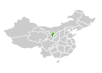
China

Ningxia
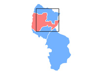
Yinchuan
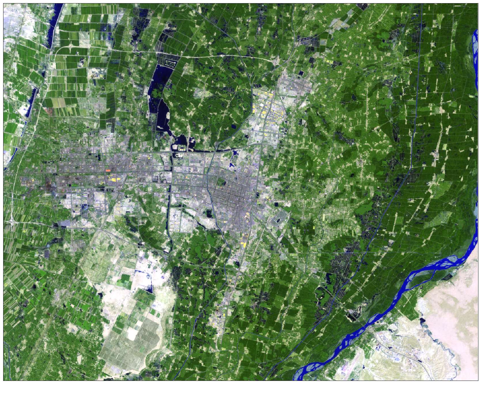
Yinchuan is the capital of the Ningxia Hui Autonomous Region in China. It has a cold desert (BWk) climate with an average yearly high temperature of 15.8°C (60.4°F) and average yearly low of 3.1°C (37.6°F). It also averages 186.3 mm (7.3 inches) of rain per year. It lies on the Ningxia plain, which the Yellow River traverses and irrigates. The administrative and commercial development of Yinchuan has been influenced by the abundance of water resources and meadowland in the surrounding area, which has facilitated the development of agriculture, aquaculture, and animal husbandry.
Data
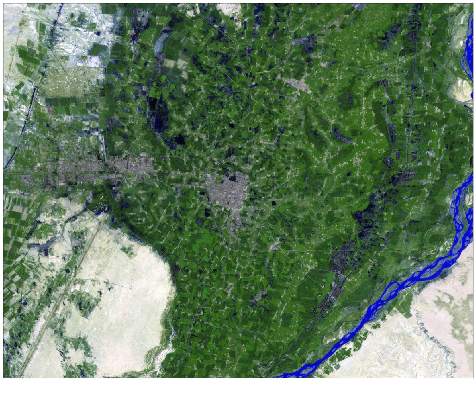
Landsat 5 TM
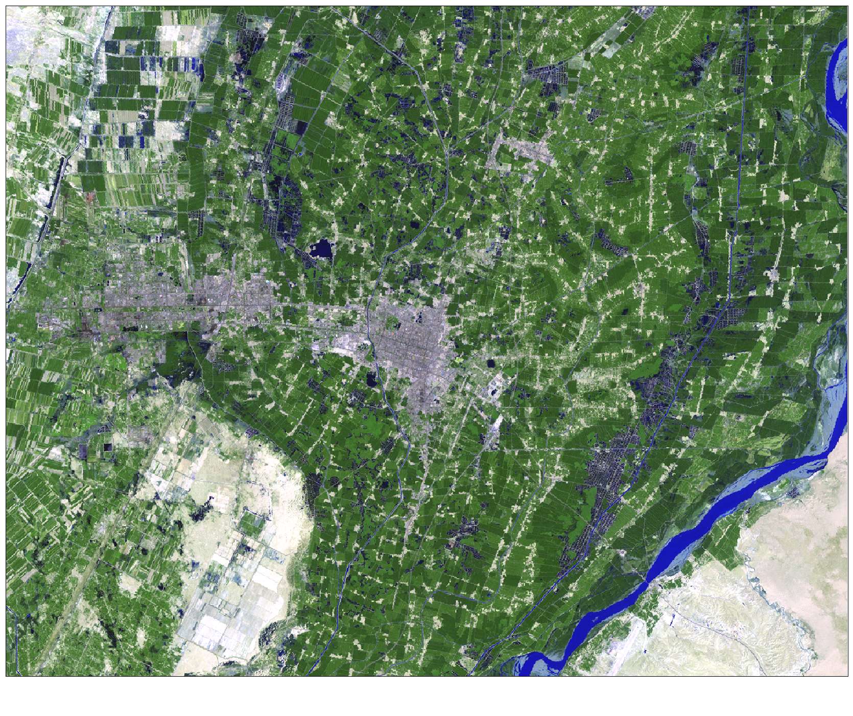
Landsat 7 ETM+
Landsat 5 TM
Landsat scenes were clipped to a rectangular study area 1400 x 1100 pixels in size to depict the area of interest. The images were determined to be well-coregistered, so no additional geometric correction was performed. The thermal band (band 6) in the 1991 image contained severe striping and was excluded during classification.
Methodology
A four class classification scheme was adopted: W = water, V = vegetation, U = urban / built-up, and P = bare field / ground. Pixels were randomly sampled for each class for each image and labeled by visual interpretation and then randomly partitioned into training and testing datasets.
| Training Samples | ||||
|---|---|---|---|---|
| W | V | U | P | TOTAL |
| 54 | 78 | 116 | 33 | 281 |
| 70 | 84 | 108 | 35 | 297 |
| 76 | 67 | 101 | 37 | 281 |
| Testing Samples | ||||
|---|---|---|---|---|
| W | V | U | P | TOTAL |
| 25 | 37 | 30 | 33 | 125 |
| 26 | 24 | 40 | 31 | 121 |
| 39 | 32 | 28 | 35 | 134 |
Using the training data, each image was initially classified by the non-contextual support vector machine (SVM) classifier, using a radial basis function (RBF) kernel in the 1-vs-1 multiclass strategy. Hyperparameters were selected by 5-fold cross validated grid search. The SVM regularization parameter C was varied in 10 steps over the range -5 to 15 in log-2 space, while the kernel bandwidth parameter G was varied in 10 steps over the range -15 to 3 in log-2 space. The parameter set yielding the highest training accuracy was selected for use at each image date.
| Date | Parameters | Support Vectors | Training Accuracy | Total Time | |||||
|---|---|---|---|---|---|---|---|---|---|
| Regularization (C) | Bandwidth (G) | W | V | U | P | TOTAL | |||
| 1991/08/30 | 8192 | 0.0743 | 6 | 8 | 12 | 15 | 41 | 96.75% | 2 min 35 sec |
| 1999/08/12 | 77936 | 0.0313 | 7 | 13 | 22 | 18 | 60 | 90.38% | 3 min 52 sec |
| 2006/08/07 | 2048 | 0.0093 | 12 | 13 | 16 | 21 | 62 | 91.54% | 4 min 2 sec |
Each classification was used to initialize contextual classification algorithms based on the Spatial-Temporal Modeling (STM) method outlined in Liu and Cai 2012 and a spatial-temporal extension of the spatial contextual Markovian Support Vector Classifier (MSVC) proposed in Moser and Serpico 2013. Each algorithm employs the Iterated Conditional Modes (ICM) optimization method to converge to a local minimum of an energy function associated with the MAP estimate of a Markov random field (MRF) modeling of an image. The MSVC reformulates the decision rule used in the MRF as a kernel in a SVM, allowing non-linear and margin-maximized decisions to be made about the contextual information and the two classifiers to be fully integrated. The energy function of the source MRF model has spatial (\(U_{S}\)) and temporal (\(U_{T}\)) components:
\[\arg\underset{L_{i}}{\min}\left\{U\left(L_{i}|\mathbf{L}_{N\left(i\right)}\right)\right\}\]
where
\[U=U_{S}\left(L_{i}\mid\mathbf{L}_{N_{S}\left(i\right)}\right)\]\[+U_{T_{1}}\left(L_{i}\mid\mathbf{L}_{N_{T_{1}}\left(i\right)}\right)\] \[+U_{T_{2}}\left(L_{i}\mid\mathbf{L}_{N_{T_{2}}\left(i\right)}\right)\]
\[\;\;\;\;=-\beta_{1}\underset{j\in N_{S}\left( i \right)}{\sum}\mathrm{I}\left (L_{j}=L_{i}\right )\]\[-\beta_{2}\underset{j\in N_{T_{1}}\left( i \right)}{\sum}\Pr\left (L_{i}\mid L_{j}\right )+\beta_{3} \underset{j\in N_{T_{1}}\left( i \right)}{\sum}\mathrm{I}\left (L_{j}\not\Rightarrow L_{i} \right )\] \[-\beta_{4}\underset{j\in N_{T_{2}}\left( i \right)}{\sum}\Pr\left (L_{i}\mid L_{j}\right )+\beta_{5} \underset{j\in N_{T_{2}}\left( i \right)}{\sum}\mathrm{I}\left (L_{j}\not\Rightarrow L_{i} \right )\]
where \(L\) is a class label, \(i\) is a pixel, \(j\in N\left(i\right)\) are its space/time neighbors, \(\mathrm{I}\) is an indicator function, and \(\beta\) are empirically estimated coefficients.
STMSVC formulates a series of contextual features, denoted by \(\varepsilon\), which are derived from the difference in energies between two classes for each of the individual energy components above. In these two class cases, the solution of the above problem can then be reexpressed as the following kernel expansion:
\[\Delta U\left(\mathbf{x}_{i},\mathbf{L}_{N\left(i \right )} \right )=\underset{j\in\mathrm{SV}}{\sum}\alpha_{j} L_{j} K_{\mathrm{STM}} \left (\mathbf{x}_{i},\left \{\varepsilon_{i,k}\right \}_{k};\mathbf{x}_{j},\left \{\varepsilon_{j,k}\right \}_{k} \right )+b\]
where \(\mathbf{x}\) is the spectral data at pixel \(i\) or \(j\), which are instances of the training data, and \(\alpha_{j}\) and \(b\) are weights and bias in the feature space induced by the kernel \(K_{\mathrm{STM}}\), which has form:
\[K_{\mathrm{STM}} \left (\mathbf{x}_{i},\left \{\varepsilon_{i,k}\right \}_{k};\mathbf{x}_{j},\left \{\varepsilon_{j,k}\right \}_{k} \right )=K\left(\mathbf{x}_{i},\mathbf{x}_{j} \right )+\sum_{k=1}^{5}\gamma_{k}\:\varepsilon_{i,k}\:\varepsilon_{j,k}\]
where
\[\varepsilon_{i,k}=U_{k}\left(-1\mid\mathbf{L}_{N_{k}\left(i \right )} \right )-U_{k}\left(1\mid\mathbf{L}_{N_{k}\left(i \right )} \right )\]
where \(K\) is a base kernel, such as the RBF kernel, used to transform the spectral data and {-1, 1} denote the assumed two classes. The weights \(\alpha_{j}\) and bias \(b\) may be calculated using a standard SVM solver. Hence, for multiclass classification, the restriction to a two class case does not pose a problem given the typical 1-vs-1 strategy that may be adopted for the SVM. As such, the STMSVC essentially computes a series of two class MRFs for each image and determines the final class label for a pixel through a winner-takes-all voting strategy.
Results
SVM:
Accuracy: 89.38%
Accuracy: 84.03%
Accuracy: 81.89%
STM:
Accuracy: 93.85%
Accuracy: 88.54%
Accuracy: 86.97%
STMSVC:
Accuracy: 96.67%
Accuracy: 93.66%
Accuracy: 91.73%
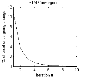
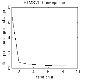
The above results are presented for the 3rd iteration of the STM algorithm and the 5th iteration of the STMSVC algorithm, which were chosen based on their maximization of the mean accuracy of the change map. Respectively, they had 1.57% and 0.47% of the total number of pixels changing class from the last iteration. Rate of convergence over 10 iterations is shown below:
Estimation by genetic algorithm yielded the following weights for the different energy contributions:
| STM | ||||||
|---|---|---|---|---|---|---|
| β0 | β1 | β2 | β3 | β4 | β5 | |
| 1991 | 1 | 2.72 | 0 | 0 | 1.78 | 0.01 |
| 1999 | 1 | 2.45 | 1.79 | 0.45 | 2.03 | 0.28 |
| 2006 | 1 | 2.61 | 1.76 | 0.12 | 0 | 0 |
The contributions are standardized based on the magnitude of the spectral coefficient, so relative interpretation between weights is possible. Hence, we see that, in all cases, the contextual information is heavily relied upon with more importance assigned to the spatial energy than the temporal energy. In the case of the 1991 image data, the temporal penalty is unimportant, whereas it shows the most importance in the 1999 image date.
| STMSVC | ||||||
|---|---|---|---|---|---|---|
| γ0 | γ1 | γ2 | γ3 | γ4 | γ5 | |
| 1991 | 1 | 0.60 | 0 | 0 | 1.20 | 1.21 |
| 1999 | 1 | 0.07 | 0.17 | 0.14 | 0.14 | 0.12 |
| 2006 | 1 | 0.70 | 0.40 | 0.02 | 0 | 0 |
The contributions are standardized based on the magnitude of the spectral coefficient, but cannot be directly compared with the STM coefficients due to the different formulation of the classifiers. Here, we see that the 1991 image data relies heavily on temporal information whereas the 1999 image data now places less importance on the contextual information. In general, we expect the spectral coefficient to be the largest here due to its relationship with the infinite-dimensional feature space induced by transformation with the RBF kernel.
Analysis
Application of the STM algorithm had the desired effects of improving single date accuracies, increasing the number of pixels with no change trajectory, decreasing the number of illogical trajectories, and decreasing the total number of change trajectories. On the other hand, application of the STMSVC algorithm had little effect on the number of pixels undergoing change and a moderate reductive effect on the number of illogical trajectories, while creating a substantial improvement in single date accuracies over STM.
Changes in the number of trajectories are listed below:
| No trajectories | Change trajectories | Illogical change trajectories | |
|---|---|---|---|
| SVM | 794,787 (51.6%) | 745,213 (48.4%) | 130,165 (8.5%) |
| STM | 991,410 (64.4%) | 548,590 (35.6%) | 71,240 (4.6%) |
| STMSVC | 813,495 (52.8%) | 726,505 (47.2%) | 97,449 (6.3%) |
The spatial pattern of change trajectories and illogical change trajectories are depicted below:
SVM:
Transitions
Illogical Transitions
STM:
Transitions
Illogical Transitions
STMSVC:
Transitions
Illogical Transitions
The above maps illustrate that application of STM had the effect of reducing misclassification noise and increasing spatial-temporal coherence. Furthermore, we can more clearly observe the spatial pattern of differences in the images due to urban, agricultural, and hydrological processes. We note that the STM algorithm may tend to oversmooth features, whereas STMSVC maintain better edge fidelity, such as is exhibited by road and highways.
References
- Burnicki, A. C., D. G. Brown, and P. Goovaerts. 2007. Simulating error propagation in land-cover change analysis: The implications of temporal dependence. Computers, Environment and Urban Systems 31(3): 282-302.
- Chang, C-C. and C-J. Lin. 2011. LIBSVM: a library for support vector machines, ACM Transactions on Intelligent Systems and Technology, 2(27), pp. 1-27. Software available at: http://www.csie.ntu.edu.tw/~cjlin/libsvm
- Congalton, R. G. and C. Green. 1999. Assessing the accuracy of remotely sensed data: Principles and practices. Boca Raton, Florida: CRC/Lewis Press.
- Liu, D. and Y. W. Chun. 2009. The effects of different classification models on error propagation in land cover change detection. International Journal of Remote Sensing 30(20): 5345-5364.
- Liu, D. and S. Cai. 2012. A spatial-temporal modeling approach to reconstructing land-cover change trajectories from multi-temporal satellite imagery. Annals of the Association of American Geographers 102(6): 1329-1347.
- Liu, D., K. Song, J. R. G. Townshend, and P. Gong. 2008. Using local transition probability models in Markov random fields for forest change detection. Remote Sensing of the Environment, 112, pp. 2222-2231.
- Melgani, F. and S. B. Serpico. 2003. A Markov random field approach to spatio-temporal contextual image classification. IEEE Transactions on Geoscience and Remote Sensing, 41(11), pp. 2478-87.
- Moser, G. and S. B. Serpico. 2013. Combining support vector machines and Markov random fields in an integrated framework for contextual image classification. IEEE Transactions on Geoscience and Remote Sensing, 51(5): 2734-2752.
- Pontius, R. G., and C. Lippitt. 2006. Can error explain map differences over time? Cartography and Geographic Information Science 33(2): 159-171.
- Tso, B. and P. M. Mather. 2009. Classification Methods for Remotely Sensed Data. Boca Raton: CRC Press.